Pick a model and run
Choose a model, then a run. New runs appear in the run list as they arrive.
Show me in the app- Open the sidebar with Edit on the toolbar, or press F1.
- On Select Data, click Model in the data type filter and click a bundle to load it.
- Click the model name near the top of the sidebar to open the model menu.
- Click a category, such as Global or Mesoscale, then click a model.
- Pick a run in the run menu next to it.
Tips
- Each model in the menu shows its latest run and a bar for how far that run has processed.
- Click the info icon next to a model for its operator, resolution, timesteps, run times and domain.
Shortcuts
- [ / ]
- Step to the previous or next run
Search models and read the availability dots
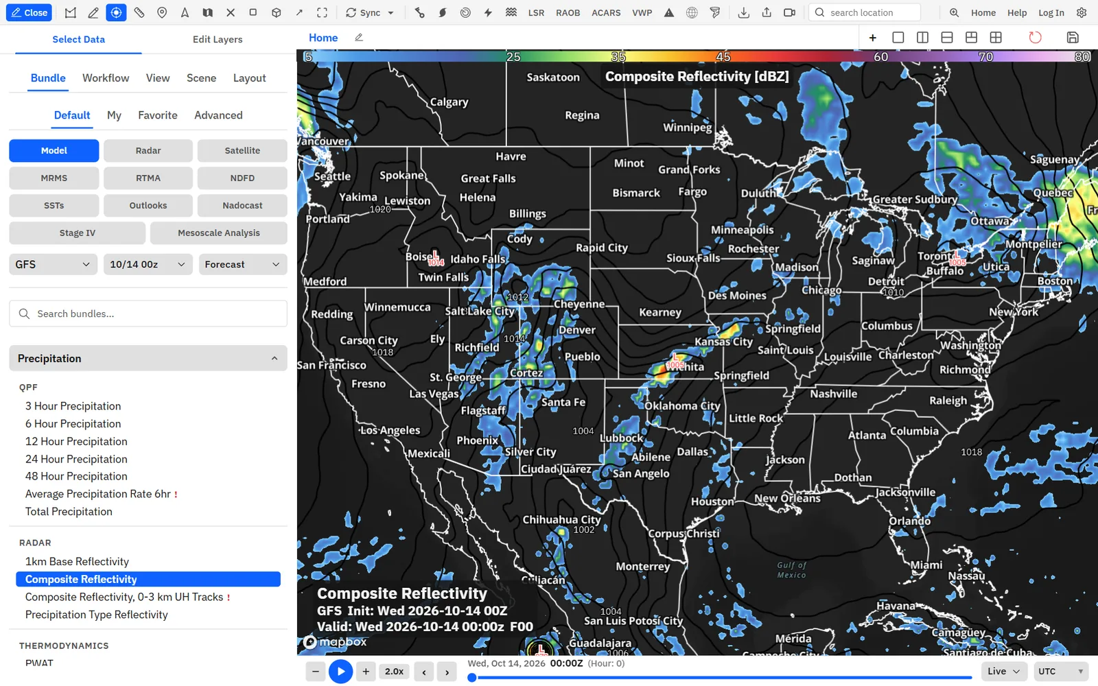
Type a model name, id or category to find a model fast. Colored dots show which models can draw the layers in your bundle.
Show me in the app- Click the model name near the top of the sidebar.
- Type a name, model id or category in Search models....
- Check the dot next to each result. Green means the model has all of your bundle’s layers, yellow some and red none.
- Click a result to switch the panel to that model.
Add a model field
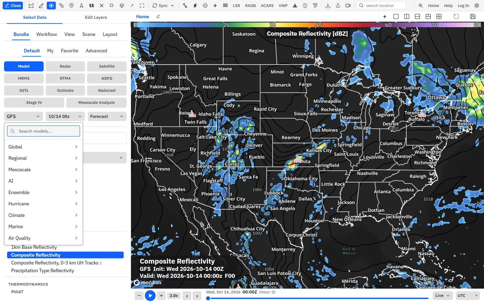
Put any field from the current model on the map, from temperature to CAPE.
- Click the Edit Layers tab in the sidebar.
- Click Add Layer.
- Click Model, then a category, then a field.
- Or type part of the name in Search variables... and click the result.
Tips
- If a field is missing, the model on the panel does not have it. Switch models and look again.
- To see which models carry a field, open Settings, choose Data, then Model, and click the field.
A bundle holds up to 8 data layers.
Trend and Compare modes
Trend keeps one valid time and steps through runs, so you can see how the forecast changed. Compare keeps one time and steps through models.
Show me in the app- Load a model bundle and move the time bar to the valid time you want.
- Open the view mode menu that reads Forecast, next to the run menu, and choose Trend.
- Drag the time bar, or use its step buttons, to move from run to run.
- For Compare, choose Compare in the same menu.
- Tick at least two models in Compare Models and click Start Comparison.
- Move the time bar to step from model to model. Choose Forecast to go back.
Tips
- Compare lists only the models that have the current run time and forecast hour.
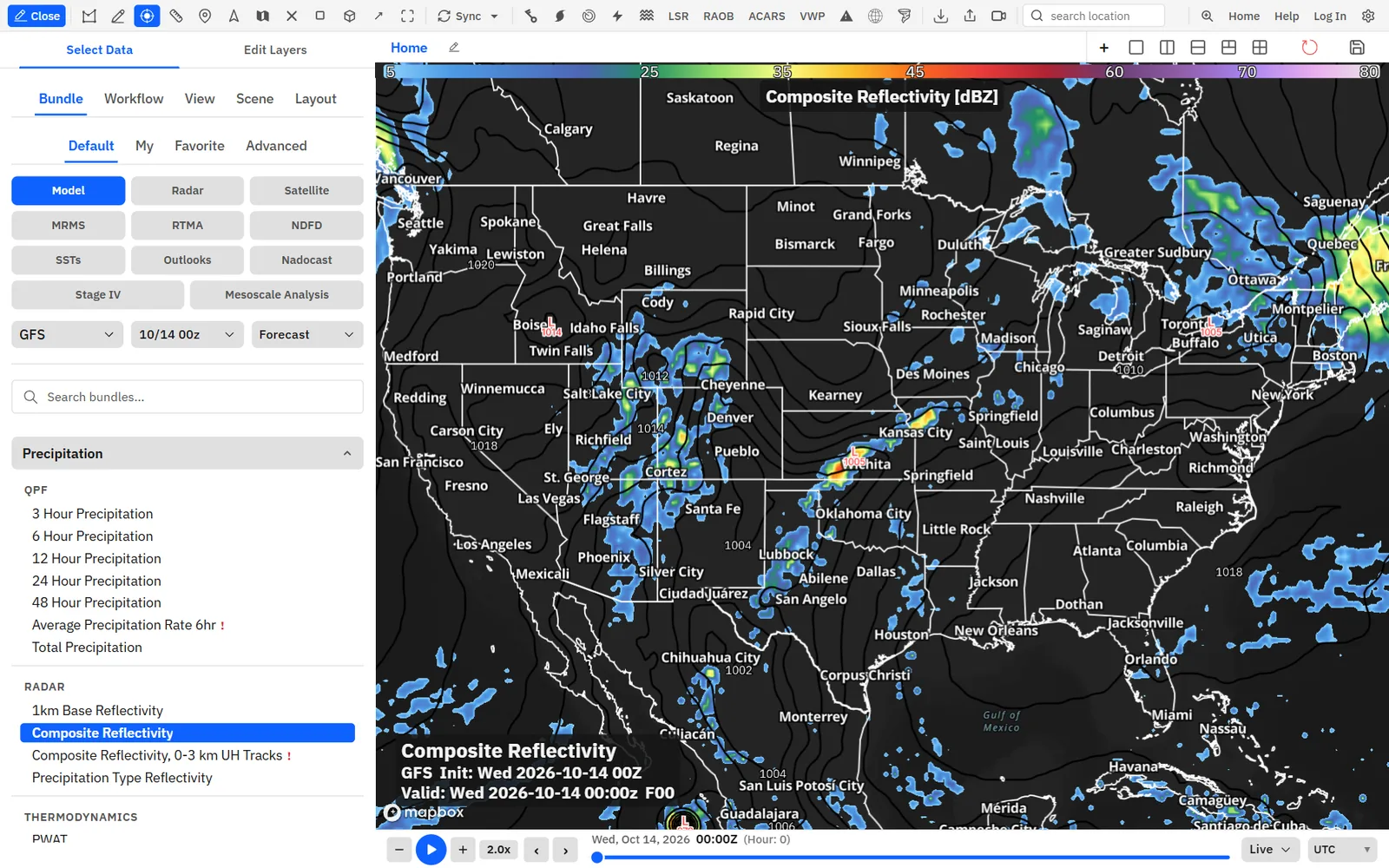
Convection-allowing models
High-resolution models that draw individual storms: HRRR and RRFS (sub-hourly too), NAM 3 km, HRDPS, NSSL MPAS, HRW FV3, WRF-ARW, ICON-D2, AROME and more.
Show me in the app- Click the model name near the top of the sidebar.
- Click Mesoscale.
- Pick a model. US models are under USA, the sub-hourly HRRR and RRFS under Sub-Hourly, and European models under European.
Free includes HRRR, HRRR Sub-Hour, RRFS A, RRFS Sub-Hour, RRFS NA and NAM 3km CONUS.
Global and regional models
GFS, ECMWF, ICON, UKMET, GDPS, ARPEGE and NAVGEM cover the world. Regional models such as NAM, RAP, RGEM, ICON-EU and ETA-CPTEC cover smaller areas.
Show me in the app- Click the model name near the top of the sidebar.
- Click Global for worldwide models or Regional for limited-area models.
- Pick a model, then a run.
Tips
- High-resolution European models such as UKV, HARMONIE and AROME-Arctic are under Mesoscale. MEPS is under Ensemble.
Free includes GFS, NAVGEM, NAM, RAP, ICON-EU and ARPEGE EU. ECMWF, ICON, UKMET and GDPS need Enthusiast or higher.
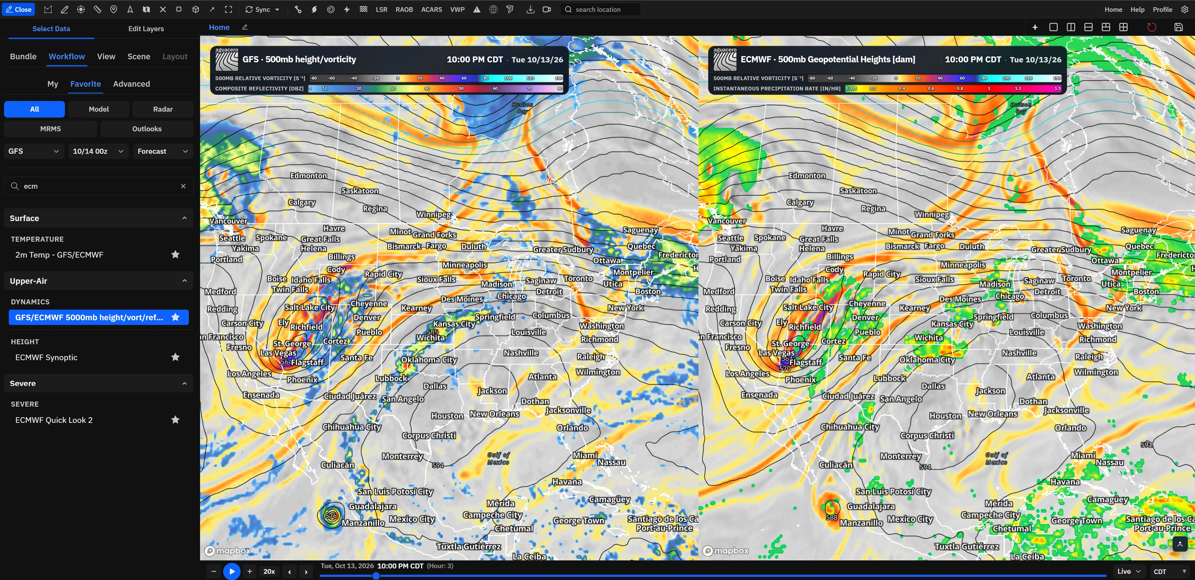
AI models
Machine-learning forecasts: ECMWF-AIFS, WeatherNext 2, AI GFS, AI GEFS, AI ICON, GEM-L, Aurora and Pangu-Weather. Several include precipitation type and snowfall.
Show me in the app- Click the model name near the top of the sidebar.
- Click AI.
- Pick a single-run model under Global or an ensemble under Ensemble.
Tips
- HRRR Cast is under Mesoscale in the same menu.
AI GFS, AI GEFS and Hybrid GEFS are on the Free plan. The other AI models need Enthusiast or higher.
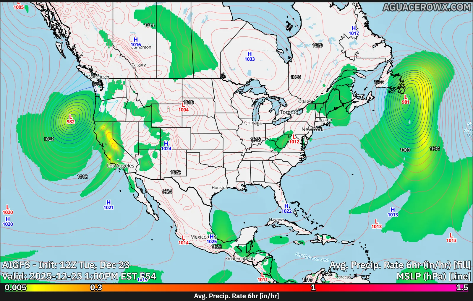
Ensembles
GEFS, GEPS, ECMWF EPS, ICON-EPS, NAEFS, MOGREPS, HREF, REFS, REPS and more, for spread and probabilities.
Show me in the app- Click the model name near the top of the sidebar.
- Click Ensemble. Global ensembles are under Global, and short-range ones such as HREF and REFS under Mesoscale.
- Pick an ensemble and a run.
- On Edit Layers, click Add Layer to add its fields, such as spread and probability products.
Tips
- ECMWF AIFS EPS and AI GEFS are in the AI menu.
GEFS, GEPS and REFS are on the Free plan.
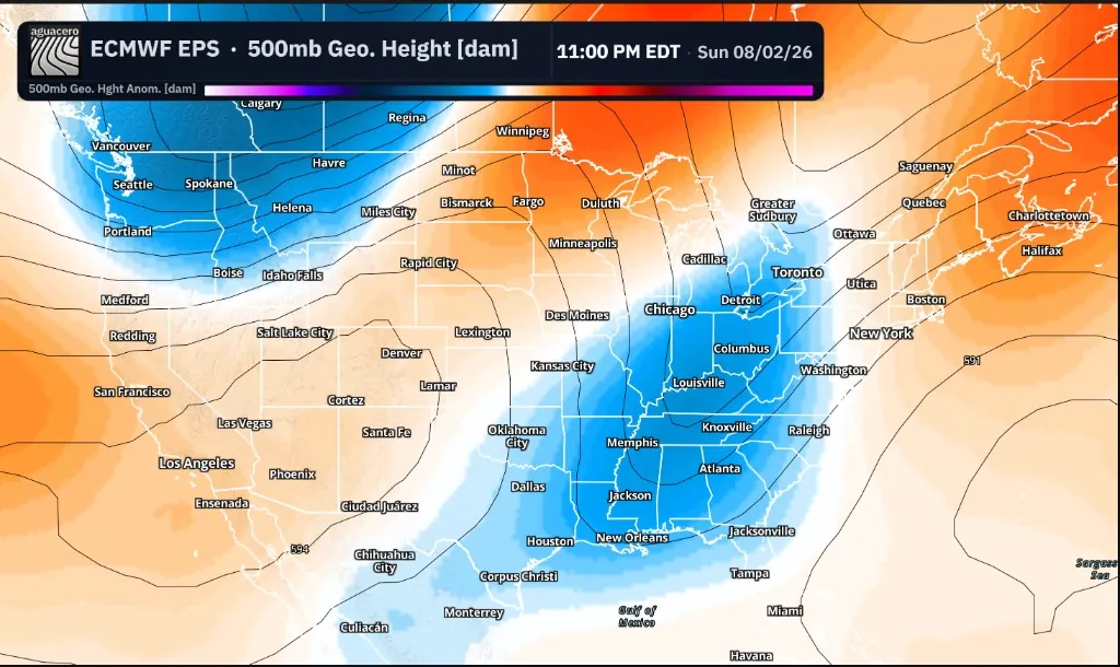
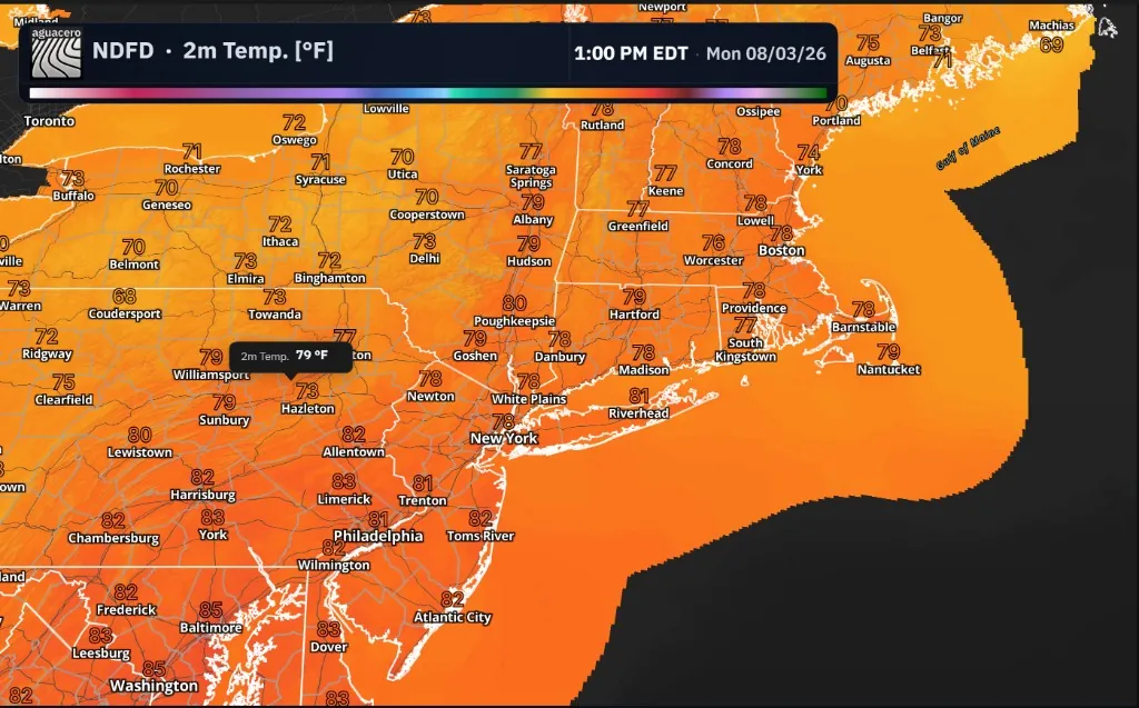
NBM and NDFDEnthusiast
The National Blend of Models every hour, and the official NWS NDFD forecast grids at 2.5 km.
Show me in the app- For the NBM, click the model name near the top of the sidebar, click Ensemble and pick NBM.
- For NDFD, click NDFD in the data type filter on Select Data.
- Click an NDFD bundle to load it.
- Pick the issuance in the NDFD run menu under the model menu.
Tips
- You can also add NDFD fields from Add Layer > NDFD.
The NBM needs Enthusiast or higher.
Severe weather parameters
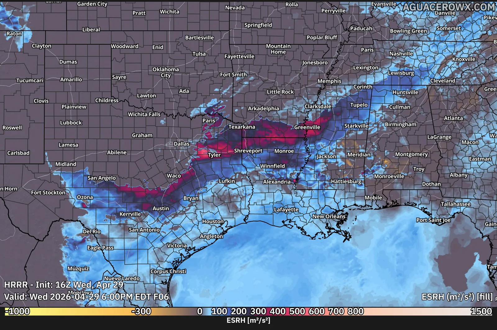
Effective SRH, SHERBE, the Violent Tornado Parameter, the Non-Supercell Tornado Parameter, downdraft CAPE, the Microburst Composite and hail fields, on the models that carry them.
Show me in the app- Switch the panel to a model with severe fields, such as the HRRR, RRFS or RAP.
- Click the Edit Layers tab, then Add Layer.
- Type a name in Search variables..., such as SHERBE, Violent Tornado, Microburst or Downdraft.
- Click the field to add it.
Winter weather fields
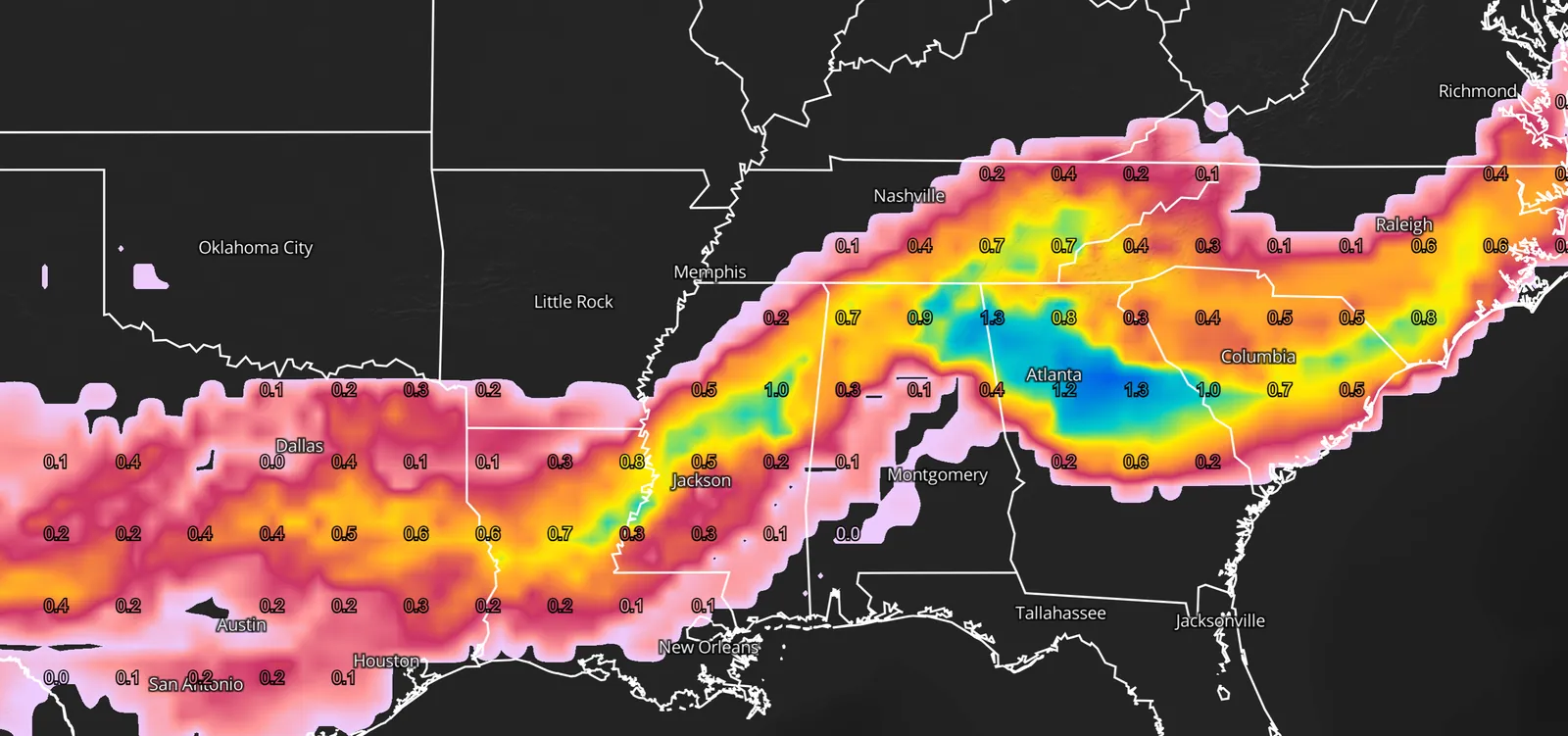
FRAM ice accumulation, precipitation-type reflectivity, snow depth change and dendritic growth zone depth.
Show me in the app- Switch the panel to a model with winter fields, such as the HRRR or NAM 3km CONUS.
- Click the Edit Layers tab, then Add Layer.
- Search for FRAM, Precipitation Type, Snow Depth Change or Dendritic.
- Click the field to add it.
Tips
- Dendritic growth zone depth is on the GFS, NAM and NAM 3 km.
Fire weather fields
The Hot-Dry-Windy Index and its anomaly, the Red Flag Threat Index and vapor pressure deficit.
Show me in the app- Switch the panel to a model with fire fields, such as the HRRR, NAM, RAP or GFS.
- Click the Edit Layers tab, then Add Layer.
- Search for Windy, Red Flag or Vapor Pressure.
- Click the field to add it.
Dynamics and isentropic analysis
Vorticity, Q-vectors, theta-e advection and moisture transport, plus wind, relative humidity and potential vorticity on the 290–330 K surfaces.
Show me in the app- Click the Edit Layers tab, then Add Layer.
- Search for Vorticity, Q-Vector, Theta-E Advection or Moisture Transport.
- For isentropic fields, switch to the GFS or NAM and search for a surface, such as 290K.
- Click a field to add it.
Anomalies
2 m temperature, 500 mb height, precipitable water and sea-level pressure anomalies against a 1991–2020 climatology.
Show me in the app- Click the Edit Layers tab, then Add Layer.
- Type Anomaly in Search variables....
- Click a field, such as 2m Temperature Anomaly or MSLP Anomaly.
Stratospheric fields
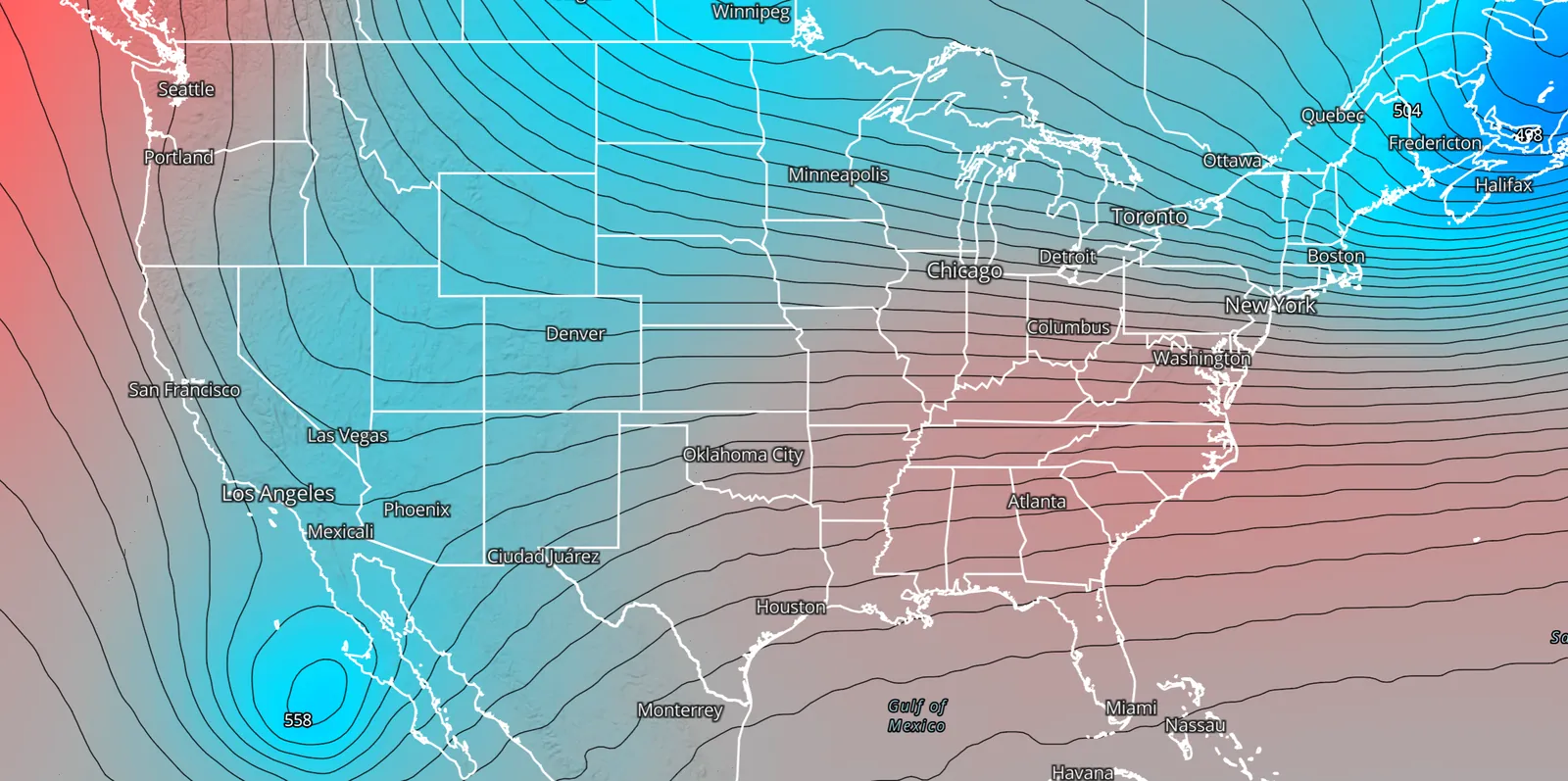
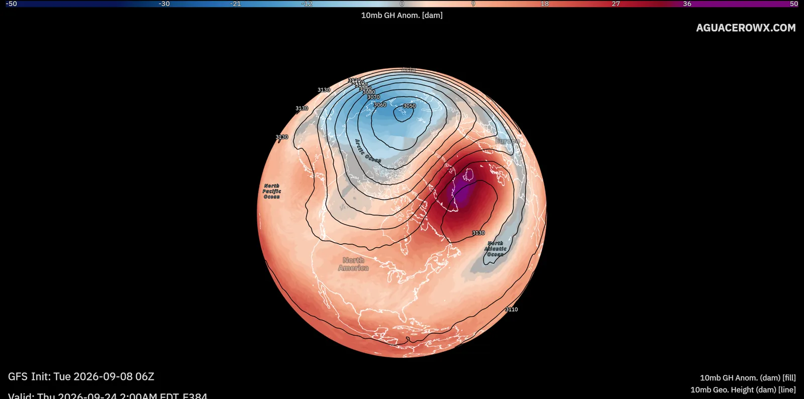
10, 50 and 100 mb temperature, height and wind on global models, with anomalies, for watching the polar vortex.
Show me in the app- Switch the panel to a global model with stratospheric fields, such as the GFS or ECMWF.
- Click the Edit Layers tab, then Add Layer.
- Search for 10mb, 50mb or 100mb.
- Click a height, temperature or wind field to add it.
Stratospheric anomalies are measured against 1990–2019 ERA5.
Air quality and smoke
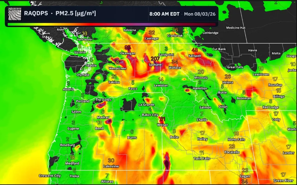
AQM, RAQDPS, CAMS Global and Regional, ICON-ART, GEFS-Aerosols, SILAM, HYSPLIT-Dust and WRF-Chem, plus smoke on supported models.
Show me in the app- Click the model name near the top of the sidebar.
- Click Air Quality and pick a model.
- On Edit Layers, click Add Layer and add a field such as PM2.5.
Tips
- For smoke on the HRRR or RAP, search Add Layer for Smoke.
AQM (AirNow) is on the Free plan.
Ocean, wave and surge models
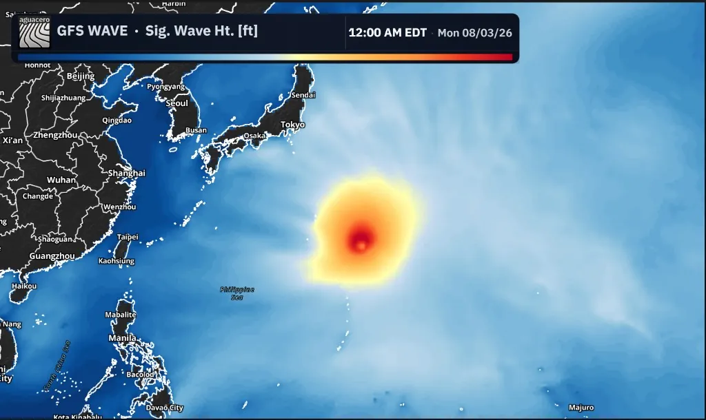
GFS Wave, ECWAM, AIFS Wave, GLWU and RTOFS, plus ETSS, P-Surge and STOFS storm surge guidance.
Show me in the app- Click the model name near the top of the sidebar.
- Click Marine.
- Pick a model under Waves, Storm Surge or Ocean.
- Add a field such as Significant Wave Height or Storm Surge from Add Layer.
GFS Wave is on the Free plan.
Seasonal and subseasonal
CFS, CanSIPS, NMME and ECMWF SEAS5 for monthly-lead outlooks.
Show me in the app- Click the model name near the top of the sidebar.
- Click Climate.
- Pick CFS, CFS Monthly, CanSIPS, NMME or SEAS5, then a run.
CFS Monthly is on the Free plan.