Open a model sounding
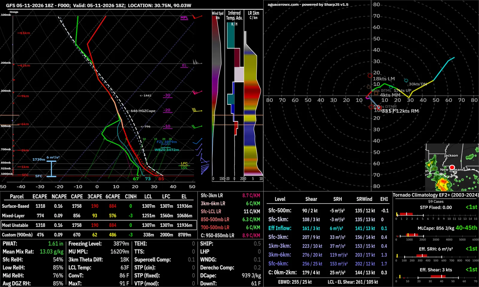
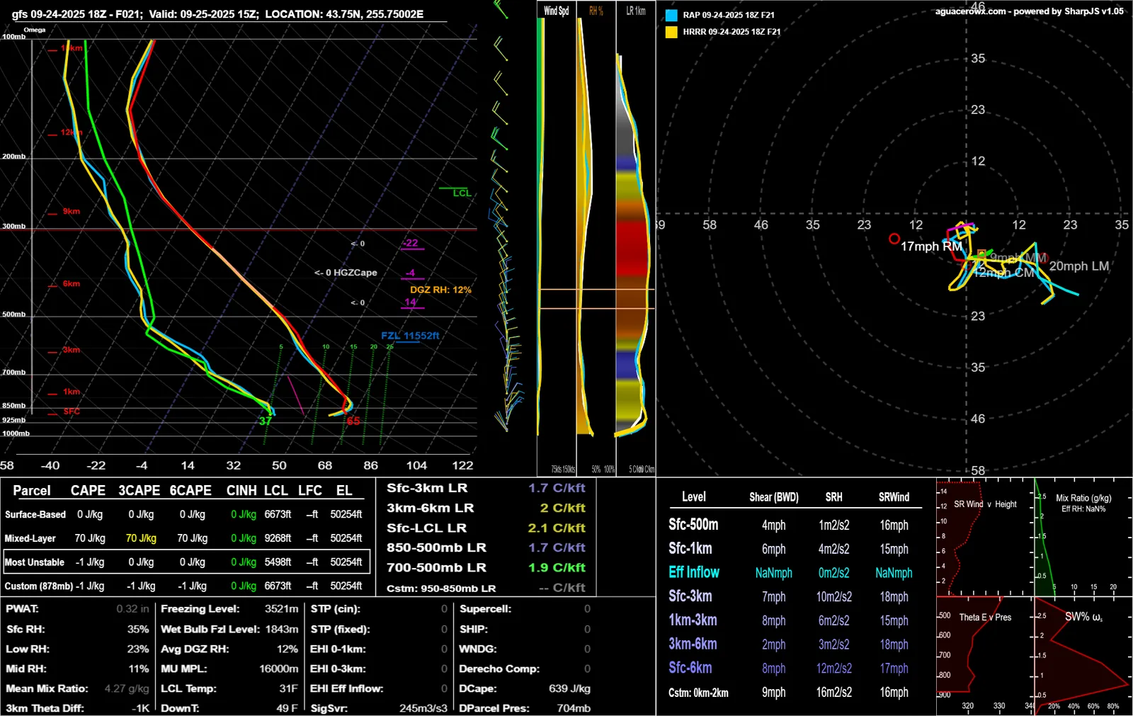
Right-click anywhere on a model map for a Skew-T with a hodograph, parcels, ECAPE and severe and winter parameters.
- Load a model bundle on the map.
- Right-click the map where you want the sounding.
- Under Soundings, click Model.
- In the controls, use Parcel Selection to switch between Surface-Based, Mixed-Layer, Most-Unstable and Custom-Pressure parcels.
- Use Storm Motion and Presets to change the storm motion, the inset parameters and the side panel view.
- Step through forecast hours with the time slider. The sounding follows it.
Tips
- Click Meso analysis instead of Model for a sounding from the SPC Mesoscale Analysis.
- Type a city, zip code, station or coordinates under Location Search and click Request Sounding to move the sounding without the map.
- Right-click the sounding to copy or download the image, or click Download Sounding Data for the data.
You can choose which items the right-click menu shows, and in what order, in Settings under Context menu.
Dock, float and resize charts
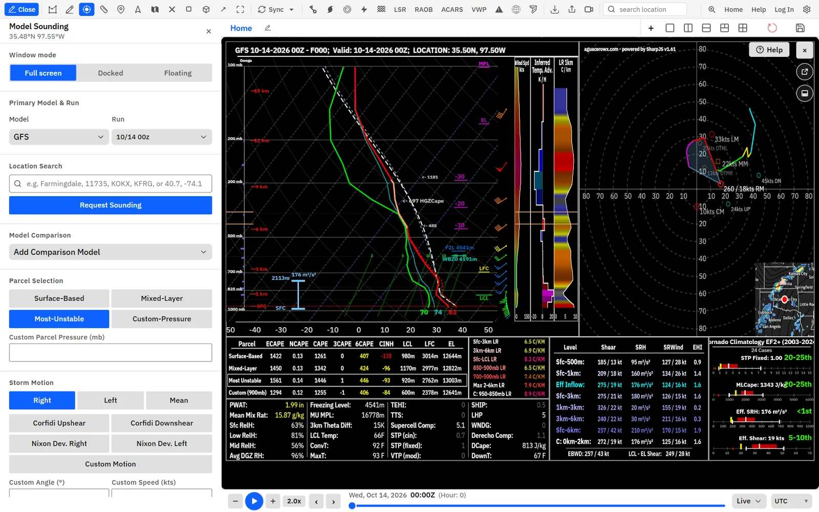
Soundings, meteograms, cross sections and VWP plots can cover the board, dock under the map or float in a window you move and resize.
- Open a sounding, meteogram, cross section image or time-height plot.
- Click the dock button on the chart (Dock under the map) to put it below the map, or the pop-out button to float it over the map.
- Drag a floating window by its title bar, and drag its edges to resize it.
- Drag the top edge of a docked chart to change its height.
- Double-click the title bar to go back to full screen.
Tips
- Window mode in the chart controls has the same three choices: Full screen, Docked and Floating.
- The app remembers the last mode you used for each kind of chart.
Docked and floating windows are on desktop only.
Draw a model cross section
Draw a line on the map for a vertical slice through the model. It stands on the map as a curtain you can drag, with presets, overlays and model-minus-model comparison.
Show me in the app- Load a model bundle on the active map.
- Click Cross section on the toolbar.
- Drag a line across the map from A to B.
- Drag the line or its A and B ends to move the cross section.
- In the controls, pick a Style preset, or choose your own Shading and Contours & wind.
- Under Model Comparison (A - B), pick a second model to plot the difference.
- Under Show as, click Image for a flat chart instead of the curtain.
Shortcuts
- Ctrl + drag
- Draw a cross section without the toolbar button
Tips
- Plot Options switches the vertical axis between height and pressure and sets the vertical exaggeration of the curtain.
- Save your own fills and overlays under Style with Save current.
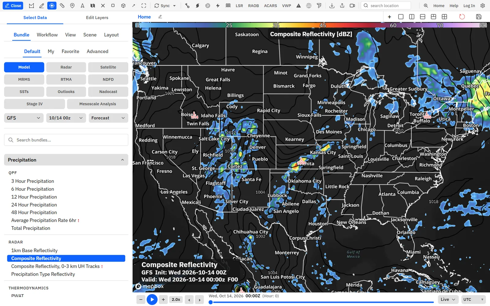
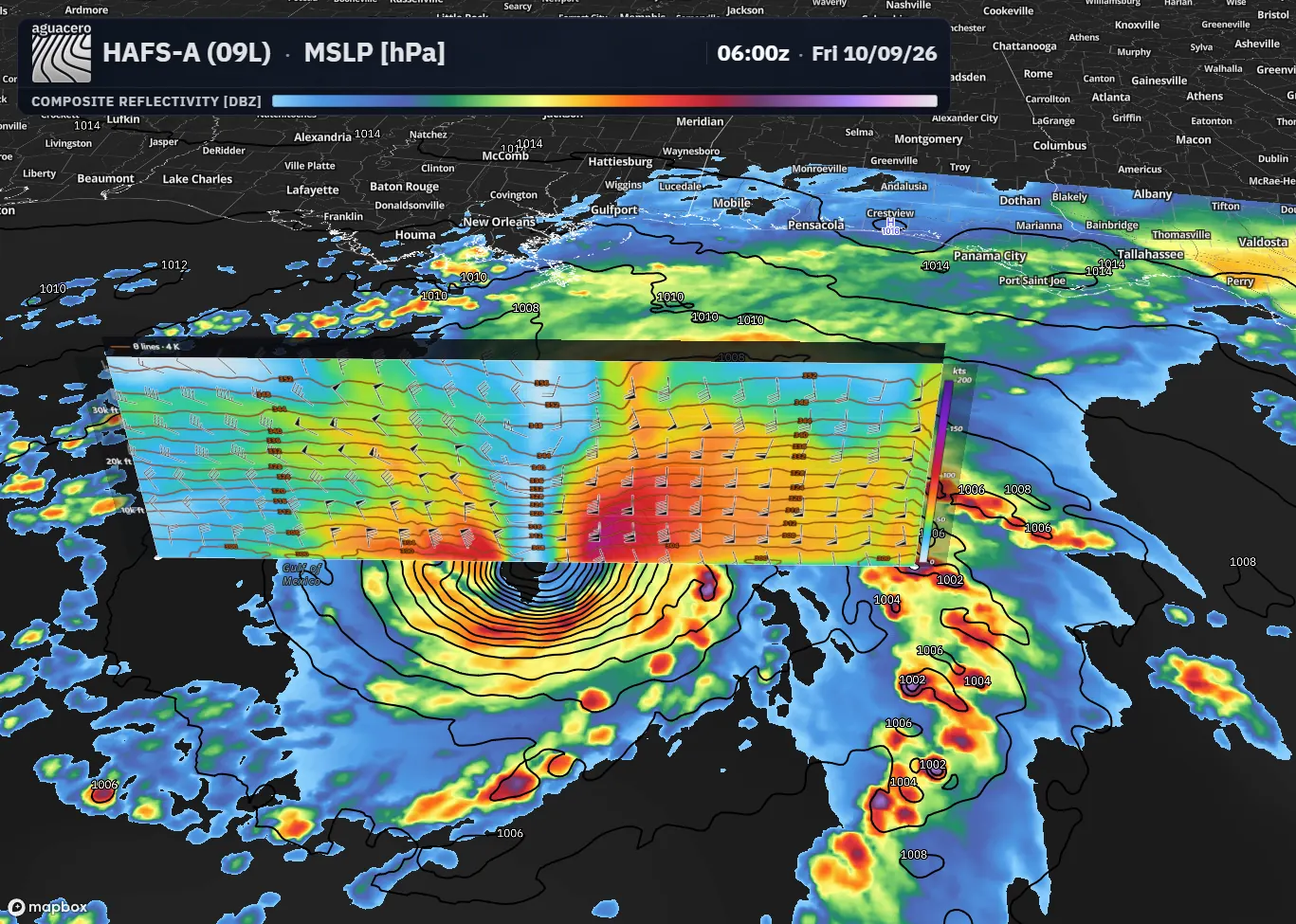
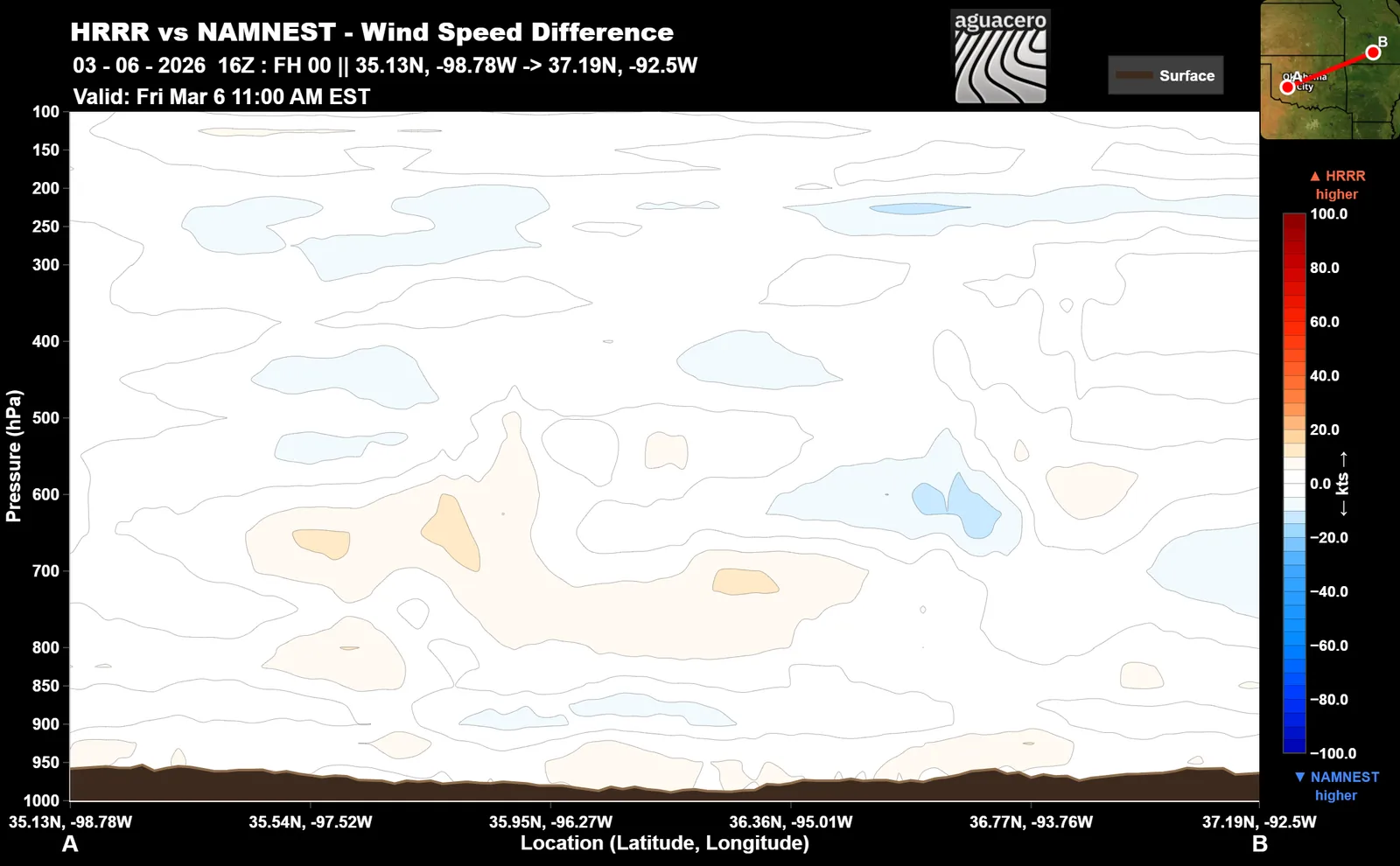
Model cross sections are on every plan. With a NEXRAD layer on the board, the same tool draws a radar cross section, which needs Professional. Compare and Trend views show the cross section as an image.
Meteograms
Temperature, dew point, wind, pressure and precipitation at one point through the model run.
- Right-click the map at the point you want.
- Under Analysis, click Meteogram.
- Use Meteogram Settings to change the Plot Layout and Precipitation Display.
- Under Model Runs, choose Comparison and click Compare Model to add models, or Trend to add earlier runs.
- Under Visualization Style, pick Line, Plume or Box.
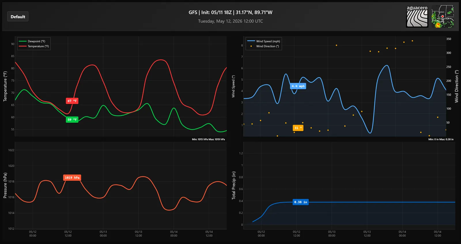
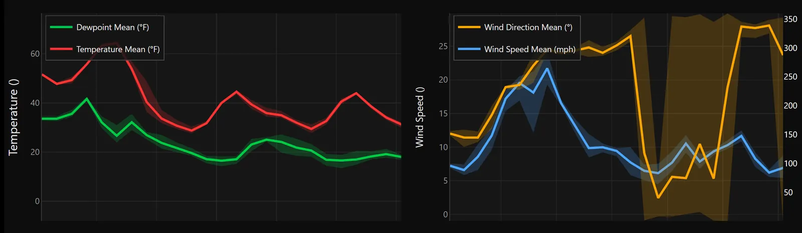
Comparison, Trend and the plume and box views need Professional.
Model time-height plots
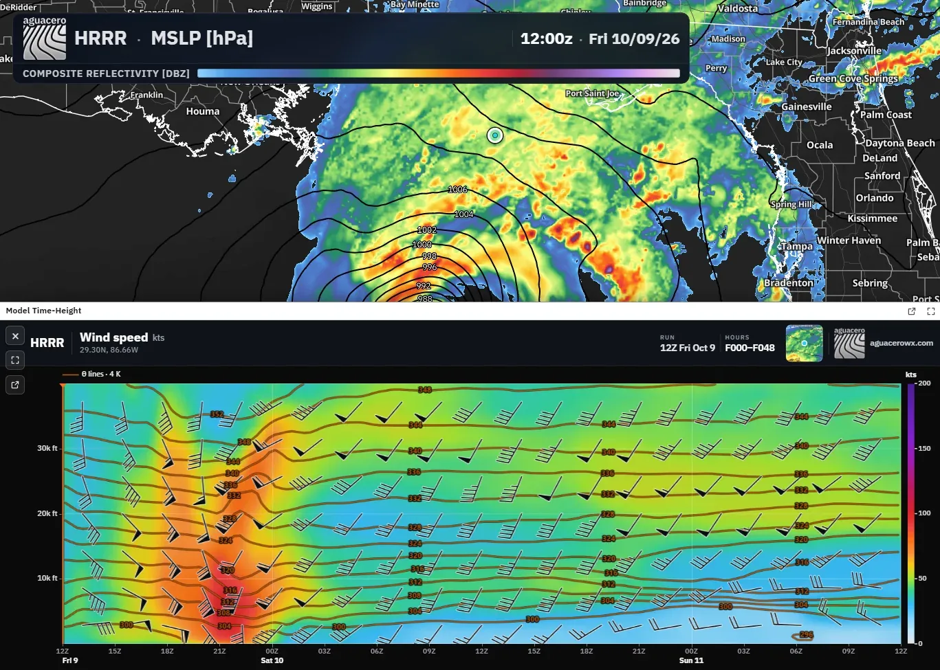
One point through the whole model run, with the same fills, barbs and contours as cross sections.
- Right-click a model map at the point you want.
- Under Analysis, click Time-height.
- Under Hours shown, pick how much of the run to plot.
- Choose fills and overlays under Style, Shading and Contours & wind.
- Drag the point on the map to move the plot, and click the chart to set the map time.
Area-averaged soundings
Draw a box for a sounding averaged over the whole area, from the model or the SPC Mesoscale Analysis.
Show me in the app- Load a model bundle on the active map.
- Click Box sounding on the toolbar.
- Drag a rectangle over the area.
- In the small menu, click Model or Meso analysis.
- Read the averaged sounding. The tool turns itself off.
Shortcuts
- Hold B + drag
- Draw a box sounding without the toolbar button
Hover soundings
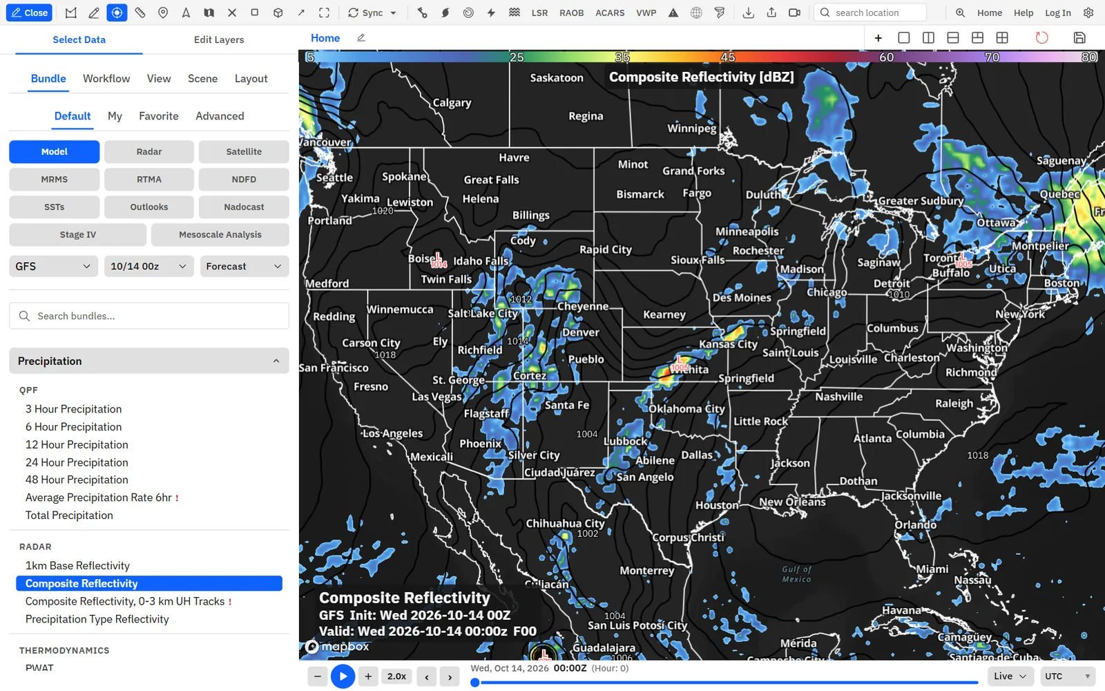
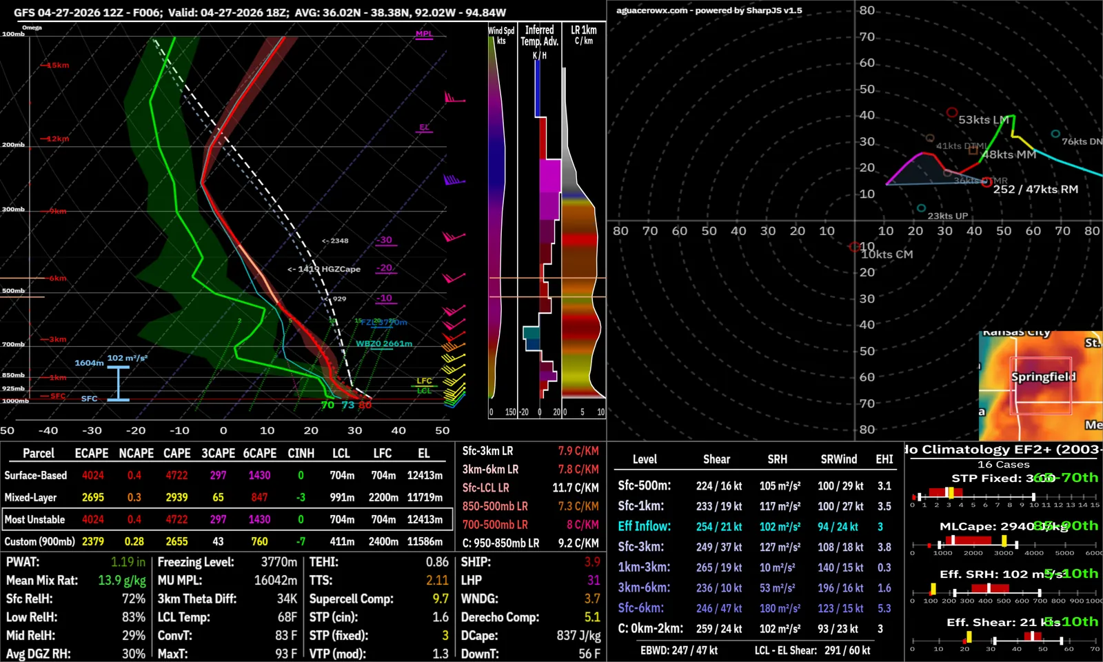
A model sounding that follows your cursor, or that you drag across the map. The profile updates as it moves.
- Right-click a model map and click Model under Soundings.
- Switch the sounding to Docked or Floating so the map stays in view.
- In the sounding title bar, click Follow mouse.
- Move the cursor over the map. The sounding updates as you go.
- Click the map to pin the sounding, and click again to follow the cursor.
- Or click Static and drag the sounding marker on the map.
Hover soundings work for model point soundings on desktop, not for RAOB, ACARS or box soundings.
RAOB soundings
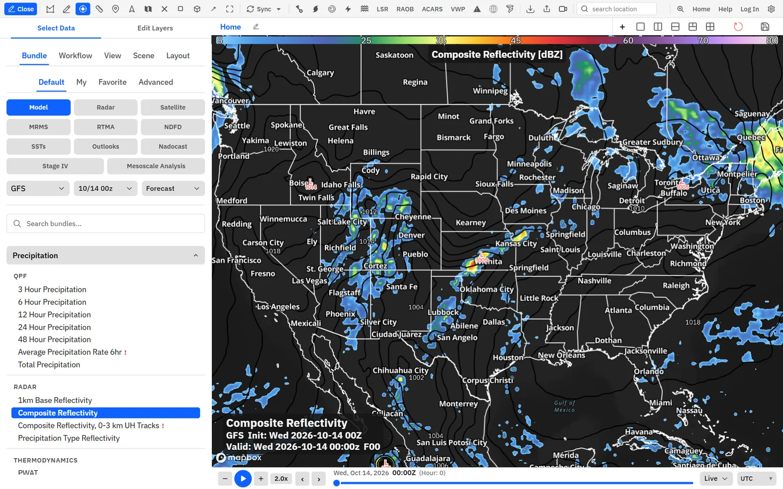
Radiosonde launch sites on the map. Click one for its observed sounding.
Show me in the app- Click RAOB on the toolbar to show the launch sites.
- Click a station on the map.
- Step through the station’s launch times with the time slider.
Tips
- Right-click the map and click RAOB under Soundings for the nearest station without turning on the sites.
ACARS aircraft soundings
Observed profiles from aircraft as they take off and land at airports.
Show me in the app- Click ACARS on the toolbar to show the airports.
- Click an airport on the map.
- Step through the airport’s soundings with the time slider.
Tips
- Right-click the map and click ACARS under Soundings for the nearest airport.
In archive mode, ACARS data goes back to January 1, 2019.
Compare soundingsProfessional
Overlay other models and runs on one Skew-T, on top of a model, RAOB or ACARS sounding.
- Open a model, RAOB or ACARS sounding.
- In the controls, under Model Comparison, click Add Comparison Model and pick a model.
- To compare runs, add the same model again, then click its row to change the run.
- Click a model’s color swatch to change its color, the eye to hide it, or × to remove it.
Tips
- To overlay your own files, use Upload Comparison Soundings under Load Custom Sounding.
Needs Professional. On other plans the button reads Compare Model (Pro).
Archived soundings
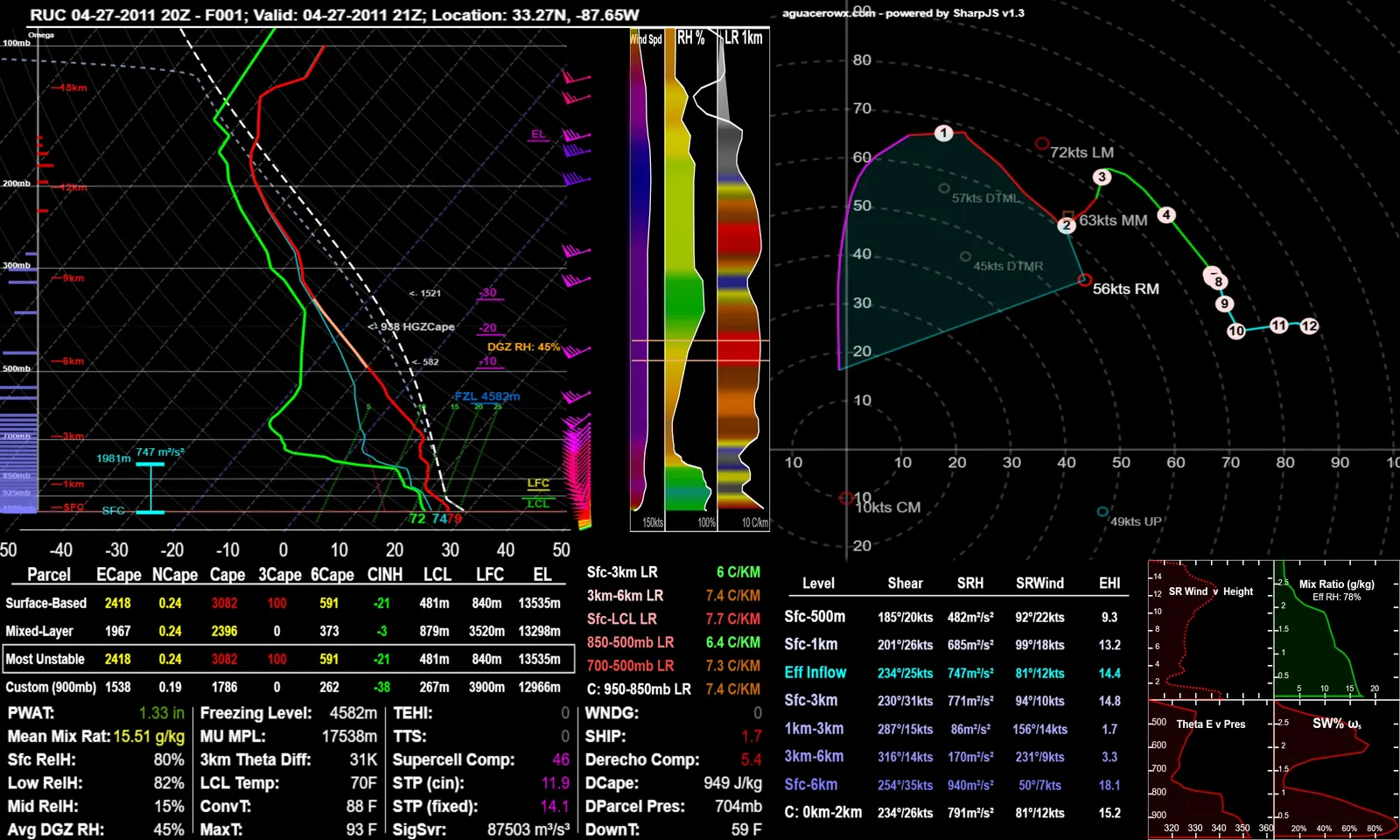
Load past RAOB, ACARS and, for select models, BUFKIT soundings for an event.
- Open any sounding.
- In the controls, scroll to Load Archived Data.
- Enter the Year:, Month: and Day:, the Station: and the Hour (Z):.
- Click Request Archived RAOB.
- For a model, set Model:, Run (Z): and Forecast Hour (Z): under Load Archived BUFKIT, then click Request Archived BUFKIT.
Tips
- Archived ACARS uses the same date with an hour and minute. Click Request ACARS.
- In archive mode, right-click and click Model to load the archived BUFKIT sounding for that point.
Hodographs on the map
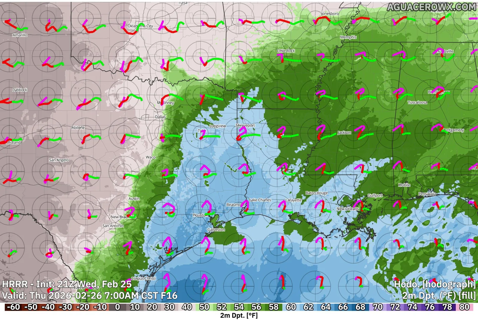
Plot hodographs across the map for select models, such as the HRRR, NAM and RAP.
Show me in the app- Load a model that has hodographs, such as the HRRR.
- Open Edit Layers in the sidebar.
- Click Add Layer.
- Open Upper Air and pick Hodograph.
- Open the layer’s settings to change the Hodograph Size and Hodograph Distance.
Shortcuts
- F1
- Open or close the sidebar
Ocean cross sections
Slice the ocean along any line: temperature to 500 m, its anomaly and its 7-, 15- and 30-day change, with the 20 °C isotherm.
Show me in the app- Load a sea surface temperature layer, for example from the SSTs data type in the sidebar.
- Click Cross section on the toolbar.
- Drag a line across the ocean.
- In Cross section type, click Ocean subsurface (ARMOR3D).
- Under Type, pick Temperature, Anomaly, 7-Day Change, 15-Day Change or 30-Day Change.
- Set the Width and Depth, and drag the A–B line to move the section.
Tips
- Click Download PNG to save the chart.